Drawing graphs and diagrams using pdfLaTeX

10 minute read

Published: November 07, 2020

In this post I have collected the options available for embedding vector graphics in LaTeX when using pdfLaTeX.

We can always use simple mathematical programs like GeoGebra for 2D and 3D graphs and drawing programs like Google Drawing for diagrams. These graphs and diagrams can be exported as png or jpg (raster graphics) and then inserted in pdf using graphicx package.

\usepackage{graphicx} %add images
\graphicspath{ {./figures/} } %images are kept in a folder under the directory of the main document.
\usepackage{subcaption} %to add multiple subfigures.

However, for better integration into the pdf document we should be using vector graphics and it can be done with the help of following programs/packages:

Software Program	dnf Package
Matplotlib	`python3-matplotlib`
Inkscape	`inkscape`

Graphs

pgfplots

For including 2D and 3D plots, we can use the pgfplots package. Read the documentation. First include the following in the preamble:

\usepackage{pgfplots} %draws function plots using pgf/tikz
\pgfplotsset{compat=1.16} %running latest version of pgfplots
\usepgfplotslibrary{external} %avoid recompiling unchanged graphs
\tikzexternalize[prefix=./figures/] %images will be stored in a folder under the working directory to avoid recompling unchanged files

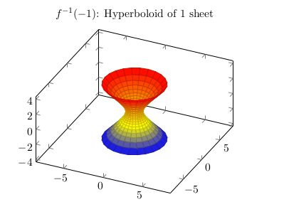
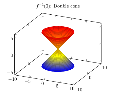
For example, we can plot 3D surfaces by following methods:

\begin{tikzpicture} %https://tex.stackexchange.com/a/359914/
\begin{axis}[title=$f^{-1}(-1)$: Hyperboloid of 1 sheet,axis equal]
\addplot3[surf,domain=0:360,y domain=-2:2] ({cosh(y)*cos(x)},{cosh(y)*sin(x)},{sinh(y)});
\end{axis}
\end{tikzpicture}

alt text

  \begin{tikzpicture}%https://tex.stackexchange.com/a/28775/
  \begin{axis}[title=$f^{-1}(0)$: Double cone, domain=0:5, y domain=0:2*pi,xmin=-10, xmax=10, ymin=-10, ymax=10, samples=20]
  \addplot3 [surf,z buffer=sort] ({x*cos(deg(y))}, {x*sin(deg(y))}, {x});
  \addplot3 [surf,z buffer=sort] ({x*cos(deg(y))}, {x*sin(deg(y))}, {-x});
  \end{axis}
  \end{tikzpicture}

alt text

The downside of this method is that it will increase the compliation time if prefix option is not used (since pdfLaTeX is limited to single CPU thread). We can also use contour gnuplot and \addplot gnuplot to extend the built-in capabilities of pgfplots by means of gnuplot’s math library, although their use is optional.

Matplotlib

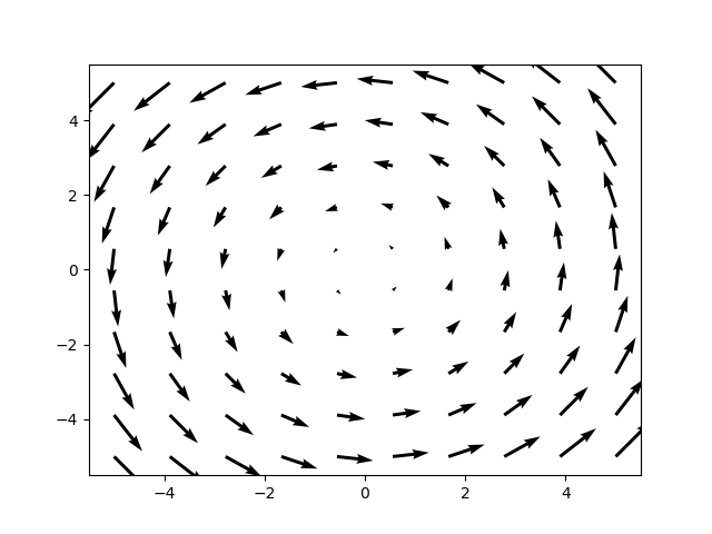
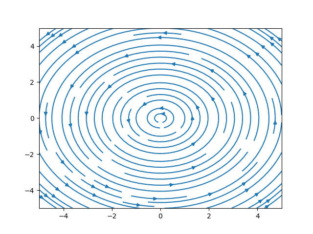
Another way of including 2D and 3D plots is to use the Python library Matplotlib. Read this guide. I will illustrate the steps involved by the following plotting the 2D vector field $X=-y\frac{\partial}{\partial x} + x\frac{\partial}{\partial y} and its flow lines:

Save and run the following Python scripts in the “figures” subfolder inside the folder containg the main LaTeX file (source1, source2):

import numpy as np
import matplotlib.pyplot as plt

#use quiver plot to plot the vector field
x,y = np.meshgrid(np.linspace(-5,5,10),np.linspace(-5,5,10))
u = -y
v = x
plt.quiver(x,y,u,v)

#save as pdf and pgf
plt.savefig('field.pdf')
plt.savefig('field.pgf')

import numpy as np
import matplotlib.pyplot as plt

#use stream plot to create the flow lines
x,y = np.meshgrid(np.linspace(-5,5,10),np.linspace(-5,5,10))
u = -y
v = x
plt.streamplot(x,y,u,v)

#save as pdf and pgf
plt.savefig('flow.pdf')
plt.savefig('flow.pgf')

Add the following lines in the preamble of the main LaTeX file:

\usepackage{pgf}
\usepackage{import} %import images from different folder 

Finally, to include pgf version of these plots in the document, use:

\resizebox{0.75\textwidth}{!}{\import{./figures/}{field.pgf}}

\resizebox{0.75\textwidth}{!}{\import{./figures/}{flow.pgf}}

You can also use figure or center environment as per your needs.

We will get the following plots with proper font and resolution:

alt text

Alternatively, you can insert the pdf file by following this guide.

Diagrams

PGF/TikZ

Manually

Apart from all these tools, one can directly use TikZ package to manually draw things like flowcharts. Read the documentation for details. For example, we can add the following to the preamble:

\usepackage{tikz}
\usetikzlibrary{shapes,arrows, chains, matrix, calc, trees, positioning, fit}
\usetikzlibrary{external}
\tikzexternalize[prefix=./figures/] %images will be stored in a folder under the working directory

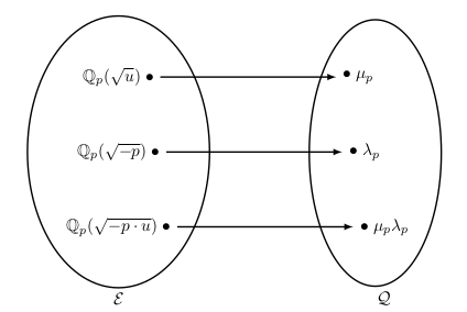
Then we can draw function mapping:

\begin{tikzpicture}[line width=1pt,>=latex]
			\node (a1) {$\mathbb{Q}_p(\sqrt{u}) \ \bullet$};
			\node[below=of a1] (a2) {$\mathbb{Q}_p(\sqrt{-p})\ \bullet$} ;
			\node[below=of a2] (a3) {$\mathbb{Q}_p(\sqrt{-p\cdot u})\ \bullet$};

			\node[right=4cm of a1] (b1) {$ \bullet \ \mu_p$};
			\node[right=4cm of a2] (b2) {$ \bullet \ \lambda_p$};
			\node[right=4cm of a3] (b3) {$ \bullet \ \mu_p\lambda_p$};

			\node[shape=ellipse, draw, minimum size=3cm,fit={(a1) (a3)}] {};
			\node[shape=ellipse, draw, minimum size=3cm,fit={(b1) (b3)}] {};

			\node[below=1cm of a3] {$\mathcal{E}$};
			\node[below=1cm of b3] {$\mathcal{Q}$};

			\draw[->] (a1) -- (b1);
			\draw[->] (a2) -- (b2);
			\draw[->] (a3) -- (b3);
\end{tikzpicture}

alt text

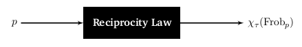
and flowcharts

\begin{tikzpicture}[>=latex']
\node[left] at (0,0) (input) {$p$};
\node[block] at (4,0) (block) [text=white]{\textbf{Reciprocity Law}};
\node at (9,0) (output) {$\chi_\tau(\Frob_p)$};
\draw[very thick, ->] (input) -- (block);
\draw[very thick, ->] (block) -- (output);
\end{tikzpicture}

alt text

Using GeoGebra Classic

The easiest way to include simple diagrams is to use GeoGebra, since it gives us the option of exporting the Graphics View as PGF/TikZ code. Installing GeoGebra Classic 6 is a dependency hell (ex1 and ex2). Therefore, we will just use the online version: https://www.geogebra.org/classic For example, add the following to the preamble:

\usepackage{pgf,tikz}
\usetikzlibrary{arrows}%you can see what extra packages are needed by going through the exported tex file

Then draw the following diagram in GeoGebra

alt text

And add the following corresponding code in the tex file:

\begin{tikzpicture}[line cap=round,line join=round,>=triangle 45,x=2.1cm,y=2.1cm]
\clip(1.5,-0.5) rectangle (10,3);
\draw (2,0)-- (4.83,0);
\draw (2,0)-- (3.41,1.41);
\draw (3.41,1.41)-- (4.83,0);
\draw (2,0.91) node[anchor=north west] {\scriptsize{$\overline{CA} \, = \, 2$}};
\draw (4.15,0.92) node[anchor=north west] {\scriptsize{$\overline{CB} \, = \, 2$}};
\draw (3.18,0) node[anchor=north west] {\scriptsize{$\overline{AB} \, = \, 2.83$}};
\draw (6,0)-- (6,1);
\draw (6,1)-- (7,1);
\draw (7,1)-- (7,0);
\draw (7,0)-- (6,0);
\draw (5.35,0.66) node[anchor=north west] {\scriptsize{$\overline{DE} \, = \, 1$}};
\draw (6.25,1.25) node[anchor=north west] {\scriptsize{$\overline{EF} \, = \, 1$}};
\draw (7.04,0.66) node[anchor=north west] {\scriptsize{$\overline{FG} \, = \, 1$}};
\draw (6.34,0) node[anchor=north west] {\scriptsize{$\overline{GD} \, = \, 1$}};
\draw (4.5,1.5)-- (5.5,1.5);
\draw (5.5,1.5)-- (5.5,2.5);
\draw (5.5,2.5)-- (4.5,1.5);
\draw (4.86,1.52) node[anchor=north west] {\scriptsize{$\overline{HI} \, = \, 1$}};
\draw (5.54,2.19) node[anchor=north west] {\scriptsize{$\overline{IJ} \, = \, 1$}};
\draw (4.25,2.2) node[anchor=north west] {\scriptsize{$\overline{JH} \, = \, 1.41$}};
\draw (7.5,1.5)-- (8.5,1.5);
\draw (8.5,1.5)-- (9.5,2.5);
\draw (9.5,2.5)-- (8.5,2.5);
\draw (8.5,2.5)-- (7.5,1.5);
\draw (8.7,2.73) node[anchor=north west] {\scriptsize{$\overline{NM} \, = \, 1$}};
\draw (9,2.08) node[anchor=north west] {\scriptsize{$\overline{ML} \, = \, 1.41$}};
\draw (7.83,1.5) node[anchor=north west] {\scriptsize{$\overline{LK} \, = \, 1$}};
\draw (7.2,2.22) node[anchor=north west] {\scriptsize{$\overline{KN} \, = \, 1.41$}};
\draw (1.94,2.51)-- (2.94,1.51);
\draw (2.94,1.51)-- (3.94,2.51);
\draw (3.94,2.51)-- (1.94,2.51);
\draw (2.8,2.76) node[anchor=north west] {\scriptsize{$\overline{OQ} \, = \, 2$}};
\draw (3.3,2) node[anchor=north west] {\scriptsize{$\overline{QP} \, = \, 1.41$}};
\draw (1.75,2) node[anchor=north west] {\scriptsize{$\overline{PO} \, = \, 1.41$}};
\begin{scriptsize}
\fill [color=black] (2,0) circle (1.5pt);
\draw[color=black] (1.9,-0.08) node {$A$};
\fill [color=black] (4.83,0) circle (1.5pt);
\draw[color=black] (4.88,-0.08) node {$B$};
\fill [color=black] (3.41,1.41) circle (1.5pt);
\draw[color=black] (3.46,1.5) node {$C$};
\fill [color=black] (6,0) circle (1.5pt);
\draw[color=black] (6.05,-0.08) node {$D$};
\fill [color=black] (6,1) circle (1.5pt);
\draw[color=black] (6.05,1.09) node {$E$};
\fill [color=black] (7,1) circle (1.5pt);
\draw[color=black] (7.04,1.09) node {$F$};
\fill [color=black] (7,0) circle (1.5pt);
\draw[color=black] (7.05,-0.08) node {$G$};
\fill [color=black] (4.5,1.5) circle (1.5pt);
\draw[color=black] (4.4,1.4) node {$H$};
\fill [color=black] (5.5,1.5) circle (1.5pt);
\draw[color=black] (5.63,1.4) node {$I$};
\fill [color=black] (5.5,2.5) circle (1.5pt);
\draw[color=black] (5.53,2.6) node {$J$};
\fill [color=black] (7.5,1.5) circle (1.5pt);
\draw[color=black] (7.45,1.4) node {$K$};
\fill [color=black] (8.5,1.5) circle (1.5pt);
\draw[color=black] (8.65,1.4) node {$L$};
\fill [color=black] (9.5,2.5) circle (1.5pt);
\draw[color=black] (9.6,2.58) node {$M$};
\fill [color=black] (8.5,2.5) circle (1.5pt);
\draw[color=black] (8.45,2.58) node {$N$};
\fill [color=black] (1.99,2.51) circle (1.5pt);
\draw[color=black] (1.99,2.59) node {$O$};
\fill [color=black] (2.94,1.51) circle (1.5pt);
\draw[color=black] (2.99,1.45) node {$P$};
\fill [color=black] (3.94,2.51) circle (1.5pt);
\draw[color=black] (3.99,2.59) node {$Q$};
\fill [color=black] (2.94,2.51) circle (1.5pt);
\fill [color=black] (2.71,0.71) circle (1.5pt);
\fill [color=black] (4.12,0.71) circle (1.5pt);
\fill [color=black] (3.41,0) circle (1.5pt);
\end{scriptsize}
\end{tikzpicture}

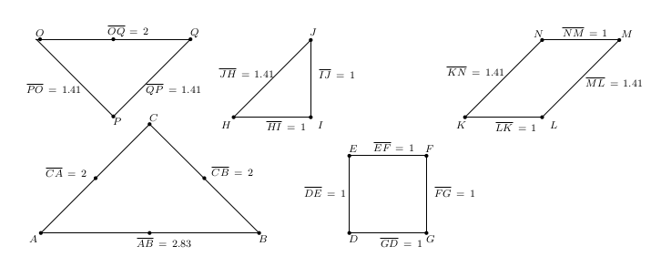
Another example, where this approach makes the job easy is the following:

alt text

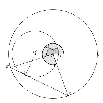
Just add this code generated by GeoGebra:

\begin{tikzpicture}[line cap=round,line join=round,>=triangle 45,x=0.75cm,y=0.75cm]
\clip(2.5,-5.5) rectangle (13.5,5.5);
\draw [shift={(8,0)},fill=black,fill opacity=0.1] (0,0) -- (0:1.2) arc (0:289.87:1.2) -- cycle;
\draw [shift={(8,0)},fill=black,fill opacity=0.1] (0,0) -- (0:0.7) arc (0:197.97:0.7) -- cycle;
\draw(8,0) circle (3.75cm);
\draw(6,0) circle (1.95cm);
\draw (8,0)-- (3.24,-1.54);
\draw (3.24,-1.54)-- (9.7,-4.7);
\draw (9.7,-4.7)-- (8,0);
\draw [dash pattern=on 3pt off 3pt] (6,0)-- (4.93,-2.37);
\draw [dash pattern=on 3pt off 3pt] (6,0)-- (13,0);
\draw [shift={(8,0)},->] (0:1.2) arc (0:289.87:1.2);
\draw [shift={(8,0)},->] (0:0.7) arc (0:197.97:0.7);
\begin{scriptsize}
\fill [color=black] (8,0) circle (1.5pt);
\draw[color=black] (7.8,-0.2) node {$O$};
\fill [color=black] (13,0) circle (1.5pt);
\draw[color=black] (13.18,-0.12) node {$B$};
\fill [color=black] (6,0) circle (1.5pt);
\draw[color=black] (5.98,0.25) node {$O'$};
\fill [color=black] (8.6,-0.08) circle (1.5pt);
\draw[color=black] (8.74,-0.22) node {$D$};
\fill [color=black] (3.24,-1.54) circle (1.5pt);
\draw[color=black] (2.94,-1.4) node {$E'$};
\fill [color=black] (9.7,-4.7) circle (1.5pt);
\draw[color=black] (9.84,-4.44) node {$E_1'$};
\fill [color=black] (4.93,-2.37) circle (1.5pt);
\draw[color=black] (4.82,-2.08) node {$G'$};
\draw[color=black] (7.5,0.8) node {$2\theta_1'$};
\draw[color=black] (8.1,0.4) node {$2\theta_0'$};
\end{scriptsize}
\end{tikzpicture}

tikz-cd

Manually

We can draw commutative diagrams using tikz-cd package. Read its documentation for details. Firstly you will have to add the following to the preamble:

\usepackage{tikz-cd}

%%homebrewcommands

\newcommand{\delbar}{\overline{\partial}}
\newcommand{\Om}{\Omega}
\newcommand{\mz}{\mathcal{Z}}

\DeclareMathOperator{\ceco}{\check{H}}

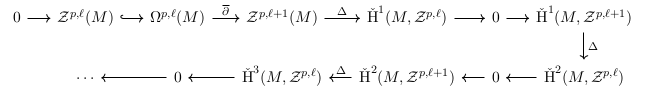
Then add the following code:

\[\begin{tikzcd}[column sep = 1.5em]
0\arrow{r} & \mz^{p,\ell}(M) \arrow[hookrightarrow]{r} & \Om^{p,\ell}(M) \arrow{r}{\delbar} & \mz^{p,\ell+1}(M) \arrow{r}{\Delta} & \ceco^1(M,\mz^{p,\ell}) \arrow{r} & 0 \arrow{r} & \ceco^1(M,\mz^{p,\ell+1}) \arrow{d}{\Delta}\\
& \cdots & 0\arrow{l} & \ceco^3(M,\mz^{p,\ell}) \arrow{l}& \ceco^2(M,\mz^{p,\ell+1})\arrow{l}[swap]{\Delta} & 0 \arrow{l} & \ceco^2(M,\mz^{p,\ell})\arrow{l}
\end{tikzcd}\]

to get

alt text

Using quiver app

The easiest way to include commutative diagrams is by using quiver app available online at https://q.uiver.app/ For example, add the following to the preamble:

\usepackage{tikz-cd}

Then draw the following diagram using quiver app

alt text

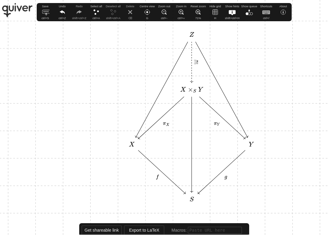
And add the corresponding exported code in the tex file:

\[\begin{tikzcd}
	&& {Z} \\
	\\
	&& {X\times_S Y} \\
	\\
	{X} &&&& {Y} \\
	\\
	&& {S}
	\arrow[from=1-3, to=5-1]
	\arrow[from=1-3, to=5-5]
	\arrow["{f}"', from=5-1, to=7-3]
	\arrow["{g}", from=5-5, to=7-3]
	\arrow[from=3-3, to=7-3]
	\arrow["{\exists !}", from=1-3, to=3-3, dashed]
	\arrow["{\pi_X}", from=3-3, to=5-1]
	\arrow["{\pi_Y}"', from=3-3, to=5-5]
\end{tikzcd}\]

Inkscape

The easiest way to include diagrams as vector graphics is by using Inkscape as follows:

Draw the desired diagram in Inkscape, and enclose mathematical symbols in $...$ . If you don’t know how to use Inkscape then just go to Help > Tutorials > Inkscape: Basic and you will be ready to use.
Create a folder called “pictures” inside the folder containg the main tex file and save the diagram as svg so that you can edit it in the future if needed. Then also save PDF+LaTeX output to the same “pictures” folder: File > Save As... > Select PDF from the drop-down menu > Click Save > Choose the following options

alt text

You can also use command-line to achieve the same result:

inkscape mySVGinputFile.svg --export-area-drawing --batch-process --export-type=pdf --export-filename=output.pdf

Add the following code to the preamble of your main tex file (source1 and source2):

\usepackage{import} % it will enable us to access images without keeping them in the document's directory
\usepackage{calc} % enable usage of \svgscale
\usepackage{graphicx} % for inserting images
\usepackage{xcolor} % for adding colors
\usepackage{transparent} % enables usage of separate color stack for transparency

Now we can add “image.svg” in one of the following ways (source1 and source2):

\begin{figure}[h]
\centering
\resizebox{75mm}{!}{\import{./figures/}{image.pdf_tex}}
\caption{Your figure}
\label{figure:example}
\end{figure}


\begin{figure}[h]
 \centering
\def\svgwidth{0.75\columnwidth}                 %Using \def\svgwidth{desired width} instead of \resizebox will preserve the font size
\import{./figures/}{image.pdf_tex}
\caption{Your figure}
\label{figure:example}
\end{figure}


\begin{figure}[h]
\centering
\def\svgscale{0.75}
\import{./figures/}{image.pdf_tex}
\caption{Your figure}
\label{figure:example}
\end{figure}

You can also write scripts to make this process easier. The main advantage of Inkscape is that there’s hardly any command or action that is impossible to do from keyboard. Linux users may not get the expected results with the key combinations starting with Alt key if the Window Manager catches those key events before they reach the inkscape application. One solution would be to change the WM’s configuration accordingly.

Gaurish Korpal

Drawing graphs and diagrams using pdfLaTeX

Graphs

pgfplots

Matplotlib

Diagrams

PGF/TikZ

Manually

Using GeoGebra Classic

tikz-cd

Manually

Using quiver app

Inkscape

You May Also Enjoy

Learning Computer Science Basics

Reading and annotating papers

Higher Arithmetic Computations

Using Terminal Emulator as LaTeX editor