Higher Arithmetic Computations
Published:
In this post, I discuss the options available for doing computational experiments in advanced number theory.
The free rein of proprietary softwares
In the world of (abstract) mathematical computations, proprietary softwares tend to be more advanced than the open source alternatives. This is mainly because of the lack of industrial support, i.e. nobody can make money by having a better abstract math computation system (see DLMF and NumFOCUS list). Following is the list of current market leaders and their open-source competitors/clones:
| Proprietary software | Speciality | Open-source alternative | Equivalent/complementary Python libraries |
|---|---|---|---|
| Desmos/TI-89 (muMATH/Derive) | Technical computations | Genius/KAlgebra/Qalculate! | Standard Library (math + decimal + fractions + turtle + tkinter + … ) |
| MATLAB (MuPAD) | Numerical computations | GNU Octave/Scilab | SciPy (NumPy + Matplotlib + …) |
| SAS/SPSS/Stata/Minitab | Statistical computations | R/Stan/PSPP/JASP | statsmodels (pandas + Patsy + Seaborn + …) |
| Maple/Mathematica (Axiom and Macsyma) | Symbolic computations (general-purpose CAS) | Maxima/FriCAS | SymPy (mpmath + Matplotlib + …) |
| Magma (Cayley + KANT V4) | Structural computations (specialized CAS for mathematical structures from abstract algebra, algebraic geometry, and finite incidence geometry) | OSCAR (GAP + Nemo + Polymake + Singular) | SageMath (CyPari2 + fpylll + JuPyMake + PySingular + Pynac + sagetex + SymEngine.py + …) |
However, closed-source projects tend to die in a decade or two (see the comments by Tim Daly). For up-to-date information, check out ISSAC (SIGSAM), Computeralgebra-Rundbrief, ICMS, JSS, and swMATH.
I must point out that RStudio is the only open-source alternative that has been able to overtake the proprietary alternatives, mainly because statistical computations can help you make money. Moreover, though the Anaconda distribution has become the standard open-source alternative to all proprietary computational softwares, there still isn’t any Python library for “structural computations” (Galois representations, isomorphisms, counting points on varieties, etc.). I believe that this is because SageMath’s motto “building the car instead of reinventing the wheel” turned it into bloatware since they integrated other well-developed open source programs like R, FriCAS, Maxima, and SymPy using Python (the glue language of scientific computing), instead of just building the Python libraries (like CyPari2) which would act as an alternative to Magma, fulfilling the original motto “Software for Arithmetic Geometry Experimentation”. To overcome this failure, SageMath evolved into a cloud-based subscription service called CoCalc to generate revenue for funding the massive project. However, the main contributions seem to come from the developments related to the LMFDB project. It might also be useful to look at the ANTS proceedings.
Mix and match
Open-source softwares has been a lifesaver for students in countries like India, where our universities couldn’t afford the proprietary softwares. I learned numerical analysis on GNU Octave and number theory on SageMath. Note that, there exist computer algebra systems that follow the philosophy of accepting a given general-purpose programming language and extending it by a set of algebraic capabilities:
| Programming language | CAS library |
|---|---|
| C | CM (with fastECPP), CMH, ffpoly, FLINT (Arb + Antic + Calcium), GMP-ECM, IML, Msieve, msolve, PARI, SIMATH (evolved into NZMATH), Symmetrica, zn_poly |
| C++ | ASurfExt, castle, CoCoALib, eclib, flatter, fplll, gf2x, Giac/Xcas, GiNaC, Givaro, HECKE, kmGNFS, LiDIA, LinBox, NTL, polymake, primesieve, SymbolicC++, SymEngine |
| Haskell | arithmoi, computational-algebra, DoCon, hgal, mod, poly |
| Julia | Nemo (FLINT wrapper with AlbstractAlgebra, Hecke, ModularForms), Symbolics |
That is, people have tried achieving a full-fledged CAS in many other programming languages, but all of them are half-baked due to the lack of contributors. In fact, using GiNaC we can get a symbolic extension for GNU Octave (nowadays can also use SymPy) and its fork Pynac provides the backend for symbolic expressions in SageMath (before that Maxima was used). Moreover, SymEngine is planned to be used as an optional fast symbolic core for SymPy since it is much faster than Pynac and a bit faster than GiNaC. However, for doing computational experiments in higher arithmetic we will have to learn multiple languages:
Any mathematician who is serious about doing extensive computational work in algebraic number theory and arithmetic geometry is strongly urged to become familiar with all three systems [Sage, Pari, and Magma] since they all have their pros and cons. Pari is sleek and small, Magma has much unique functionality for computations in arithmetic geometry, and Sage has a wide range of functionality in most areas of mathematics, a large developer community, and much unique new code. – SageMath October 2008 Bordeaux meeting
There is similar advice from Andrew Sutherland and John Voight in this blog post by Frank Calegari.
Python: General-purpose programming language (open-source)
During my undergraduate studies, I had the perception that C++ is “the langauge” for scientific computations (see the table above). In fact, the C/C++ libraries like GMP, MPFR, and GNU MPC serve as the foundations for various other higher arithmetic computation libraries. However, with the advent of Cython (not to be confused with CPython, which is the original Python implementation), Python has become “the new langauge” for scientific computations. The key advantage of Python over C++ is that Python provides better code readability than C++ (like using whitespaces instead of curly braces). In fact, all these C/C++ libraries can now be accessed via SageMath using Python-based syntax. For example, in 2016, Robert J. Lemke Oliver used SageMath and C++ to verify the observations by Kannan Soundarajan, leading to the famous discovery of biases in the distribution of consecutive primes.
To begin the Python journey, we will need the following packages:
| Software Program | dnf Package |
|---|---|
| Python3 | python3 |
| SymPy* | python3-sympy |
| CyPARI2** | python3-cypari2 |
*Note that Fedora will automatically install the required dependecies like mpmath, Cython, matplotlib etc.
**Requires the actual PARI/GP package and the PARI library development package.
If you want GUI version of Python development environment then can get IDLE by installing the package python3-idle. We will use Vim as the text editor for writing Python scripts. Note that we don’t need to add a file extension, however for proper syntax highlighting we will use the file extension .py. Therefore, it would be helpful to install the python-mode plugin (instructions). Following are some the key mappings for some of the python-mode commands (documentation):
| Key mapping | Python-mode command (normal mode) | Output |
|---|---|---|
\\r | :PymodeRun | Run current code script buffer or selection |
| (Ctrl+w) + z | :pclose | Close the code preview window (not in doc) |
| Shift + k | :PymodeDoc | Show documentation for current word |
| Ctrl + p | Usual Vim key binding | Auto-complete a word that has already been typed once in the document |
Note that the text-wrap is disabled by default, with the maximum line length of 79 characters. Moreover, it uses pylint to check code at every save. I couldn’t figureout how to use code completion via rope.
One can learn the basics by going through Hands-on Python Tutorial by Andrew N. Harrington or skimming through the tutorial available in the official documentation. If you prefer video lectures, then the MIT OCW Introduction to Computer Science and Programming in Python is a good option (many other free tutorials are also there on YouTube).
Python is a multi-paradigm, call by object, statically scoped, both dynamically and strongly typed programming language.
Therefore, though Python is an object-oriented language, it doesn’t imply that it doesn’t support other programming paradigms (wikipedia). Also, it would be wise to keep in mind the floating point arithmetic limitations that these general purpose programming languages. For example, if using Python as a calculator, we will get “wrong” answers when using decimals:
# Python3 examples
>>> 3.3 - 1.1  # Do not depend on the exactness of floating point arithmetic, even for apparently simple expressions!
2.1999999999999997
>>> 0.1+0.2  # so here 0.3 is not equal to 0.1 + 0.2
0.30000000000000004
>>> format(.1, '.20f')  # 0.1 does not has exact representation in binary floating point
'0.10000000000000000555'
To familiarize yourself with the useful maths libraries in Python (for example, mpmath provides support for arbitrary-precision floating point arithmetic, one can use the notes for the Maths with Python course at the University of Southampton or Fundamentals of Computer Programming course by Clinton Bradford at Purdue University. If you prefer video lectures, then the MIT OCW Introduction to Computational Thinking and Data Science is a good option. For example, we can get “correct” answers for float arithmetic by using decimal module:
# trying to bypass float arithmetic problem
>>> from decimal import *
>>> Decimal('3.3') - Decimal('1.1')
Decimal('2.2')
>>> Decimal('0.1') + Decimal('0.2')
Decimal('0.3')
>>> Decimal('0.1') == 0.1
False
>>> Decimal('3.5') == 3.5
True
Examples
For elementary numer theory examples, you can use either the course notes for this (very) short course in Number Theory by Robert Campbell at the University of Maryland, Baltimore County (course website) or the the companion website for the book “An Illustrated Theory of Numbers” by Martin H. Weissman. However, here we will take some examples from SageMath and solve them using Python libraries.
Plotting elliptic curves over affine plane
- SageMath script and output
 p=plot(EllipticCurve([0,0,0,3,0]), gridlines='true', color=hue(0.7),xmin=-4, xmax=4, ymin=-3, ymax=3, legend_label='$y^2=x^3+3x$')
 p+=plot(EllipticCurve([0,0,0,2,0]), gridlines='true', color='cornflowerblue',xmin=-4, xmax=4, ymin=-3, ymax=3, legend_label='$y^2=x^3+2x$')
 p+=plot(EllipticCurve([0,0,0,1,0]), gridlines='true', color='red',xmin=-4, xmax=4, ymin=-3, ymax=3, legend_label='$y^2=x^3+x$')
 p+=plot(EllipticCurve([0,0,0,-1,0]), gridlines='true', color='orange',xmin=-4, xmax=4, ymin=-3, ymax=3)
 p+=plot(EllipticCurve([0,0,0,-2,0]), gridlines='true', color=hue(0.2),xmin=-4, xmax=4, ymin=-3, ymax=3, legend_label='$y^2=x^3-2x$')
 p+=plot(EllipticCurve([0,0,0,-3,0]), gridlines='true', color=hue(0.3),xmin=-4, xmax=4, ymin=-3, ymax=3, legend_label='$y^2=x^3-3x$')
 p.set_legend_options(shadow=False, loc=2)
 show(p)
 p.axes_labels(['$x$','$y$'])
 p.save('ec.pdf')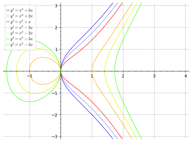
- Python script and output
- SageMath script and output
Plotting elliptic curve modulo prime
- SageMath script and output
  E=EllipticCurve(GF(1021),[0,-1,-1,0,0])
  A=E.plot()
  show(A)
  A.save('v1.pdf')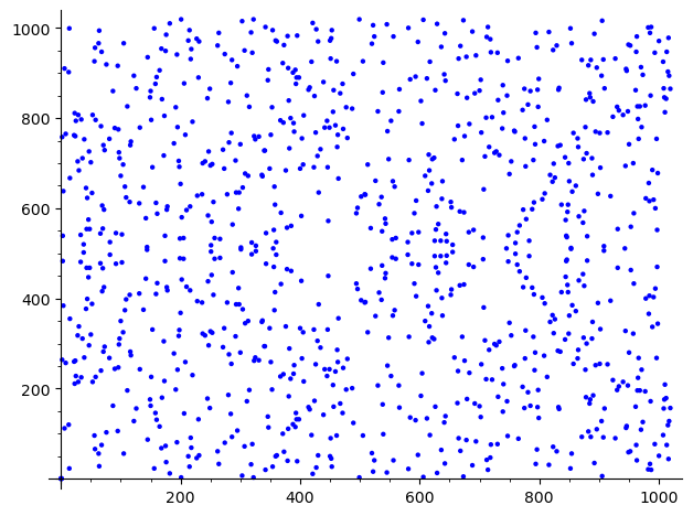
- Python script and output
Comparing the prime counting functions
- SageMath script and output
 P = plot(Li(x), (x,2,10000), linestyle="--", thickness=2, rgbcolor=(0,0,0), legend_label='$\\mathrm{Li}(x)$')
 Q = plot(prime_pi(x), (x,2,10000),thickness=2, rgbcolor=(0,0,0), legend_label='$\\pi(x)$')
 R = plot(x/log(x), (x,2,10000), linestyle=":", thickness=3, rgbcolor=(0,0,0), legend_label='$x/\\log(x)$')
 (P+Q+R)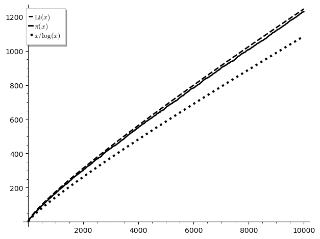
- Python script and output
Plotting Riemann zeta function for real inputs (trivial zeros)
- SageMath script and output
  p=plot(zeta(x), (x,-13,-1), legend_label='$\\zeta(x)$')
  show(p)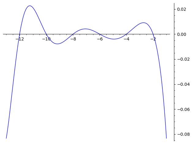
- Python script and output
Plotting the real and imaginary parts of the Riemann zeta function $\zeta(1/2 + it)$ for $0 < t < 30$
- SageMath script and output
  i = CDF.gen()
  v = [zeta(0.5 + n/10 * i) for n in range(300)]
  L = [(z.real(), z.imag()) for z in v]
  line(L)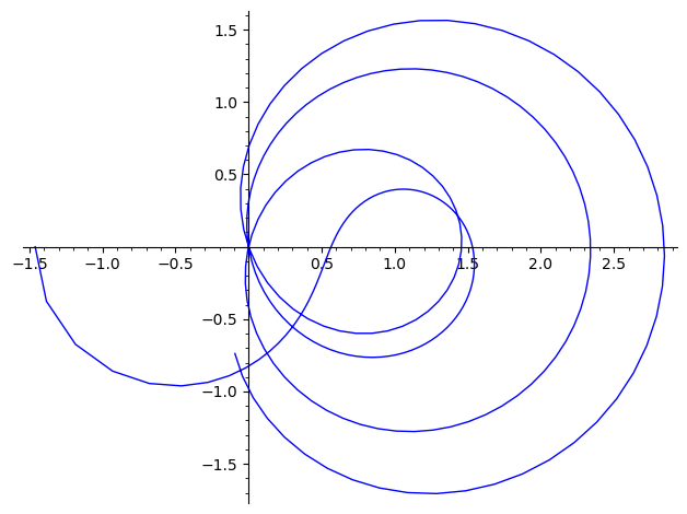
Comparing the argument and absolute values of Riemann zeta function $\zeta(1/2 + it)$ for $0 \leq t \leq 50$
- SageMath script and output
  i = CDF.0
  p1 = plot(lambda t:  arg(zeta(0.5+t*i)), 1, 50,linestyle="--", rgbcolor=(0,0,0), legend_label='$\\mathrm{arg}(\\zeta(0.5+it))$')
  p2 = plot(lambda t:  abs(zeta(0.5+t*i)), 1, 50, rgbcolor=(0,0,0), legend_label='$|\\zeta(0.5+it)|$')
  p1+p2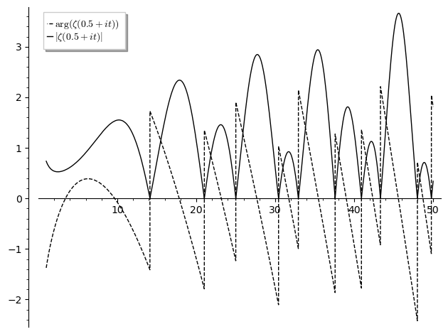
Plotting complex valued functions
- SageMath script and output
complex_plot(x^4-1,(-5,5),(-5,5))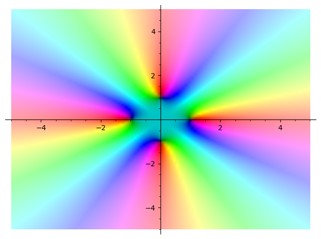
Ideal factorization
- SageMath script and output
  K.<a>=NumberField(x^3-19)
  I = K.ideal(3)
  F = I.factor()
  F
(Fractional ideal (3, 1/3*a^2 + 1/3*a + 1/3))^2 * (Fractional ideal (3, 1/3*a^2 + 1/3*a - 2/3))- Python script and output
Magma: Domain-specific programming language (proprietary)
There exist individual C/C++ libraries, like FLINT and m4ri, which are much more efficient than Magma. In fact, Magma itself uses some of the C/C++ libraries like ATLAS, GMP, GMP-ECM, MPC, and MPFR. However, there aren’t enough libraries available to enable SageMath completely replace Magma.
In the USA, because of the Simons Foundation Agreement, you can get access to Magma for free by contacting your department’s IT support staff. You should be able to access its full-version on your department’s computer clusters and student-version on your personal computer (installation steps). Note that the student-version is available only for the outdated 32-bit architecture, therefore you might also need to install additonal packages like glibc.i686 in Fedora (details) or ia32-libs-multiarch in Ubuntu (details).
We will use Vim as the text editor for writing Magma scripts. Note that, just like for Python scripts, we don’t need to add any specific filename extensions to the text files in order to be able to “load them” in Magma (details). However, one can use filename extension .m to get Objective-C syntax highlighting (objc.vim) and to be consistent with the extension used for magma package files (details). Moreover, we can run the code without having to leave the text editor by adding the following to .vimrc file (source):
map <F2> :w<CR>:!magma %<CR> "once you press <F2> in normal mode, it first saves your file and then run the file with magma.
imap <F2> <Esc>:w<CR>:!magma %<CR> "once you press <F2> in insert mode, it first leaves insert mode, then saves the file and then run the file with magma.
One can learn the basics by going through the “First Steps in Magma” or skimming through the first chapter of the “Handbook of Magma Functions”, you will be ready to start using Magma for solving math problems. Note that Magma supports the old-school procedural programming paradigm with an ability to implement functional style.
Magma is an imperative, call by value, statically scoped, dynamically typed programming language, with an essentially functional subset.
Examples
For some elementary numer theory examples, see the Micro introduction into Magma available on the legacy website of Harvard University’s Department of Mathematics. However, we will take some examples from SageMath and solve them using Magma. Note that, unlike SageMath, Magma doesn’t have access to any plotting library like matplotlib. Therefore, we can’t reproduce the graphical examples we saw above.
Ideal factorization
- SageMath script and output (doc)
  K.<a>=NumberField(x^3-19)
  I = K.ideal(3)
  F = I.factor()
  F
(Fractional ideal (3, 1/3*a^2 + 1/3*a + 1/3))^2 * (Fractional ideal (3, 1/3*a^2 + 1/3*a - 2/3))- Magma script and output
  R<x>:=PolynomialRing(Integers());
  f:=x^3 - 19;
  K<y>:=NumberField(f);
  O:=MaximalOrder(K);
  I:=3*O;
  Factorization(I);
[ <Prime Ideal of O Two element generators: [3, 0, 0] [2, 0, 2], 1>, <Prime Ideal of O Two element generators: [3, 0, 0] [0, 2, 1], 2> ]
Conclusion
William Stein has played a key role in starting this open-source mathematical software revolution. For example, there exist free online textbooks which use SageMath to teach elementary number theory, linear algebra, abstract algebra, graph theory, and game theory. However, it would have been great if the academic community could understand the value of open-source Python-based Magma.
Fortunately, the OSCAR project, supported by the German Research Foundation (DFG) since January 2017, has the potential of becoming an open-source Julia-based Magma. I believe that unlike SageMath, OSCAR will be able to replace Magma, since like Magma is maintained by the Computational Algebra Group at the University of Sydney, OSCAR is maintained by the Algebra, Geometry and Computer Algebra group at TU Kaiserslautern (usecase example). Moreover, Julia has simple syntax like Python (Python equivalent is CPython: interpreted language for fast software development), is as fast as C++ (Python equivalent is Cython: compiled language for fast computations) and uses a LLVM just-in-time (JIT) compiler similar to the JVM JIT compiler of Java (Python equivalent is PyPy, similar to LuaJIT: dynamic language for fast computations).
In my opinion, the research papers funded by public taxes should be freely available (like free beer) and the softwares needed to do tax-funded research should also be freely available (like free speech). Recently, there has been a surge in researchers using SageMath or Python for doing computations in higher arithmetic. For example, this arithmetic geometry paper uses Python for computations.
